Is the stat plausible?
The first thing to check when presented with a statistic, especially out of context, is whether the claim is even vaguely reasonable.
Back of the napkin calculations
One way to check plausibility is a quick on-the-fly calculation.
Say, for example, we run into someone claiming that “in the 35 years since marijuana laws stopped being enforced in California, the number of marijuana smokers has doubled every year”.
Well, even if we start with the most generous estimate that initially there was only 1 lonely pothead in California, then if that number doubled every year for 35 years:
\[\begin{aligned} \text{Year 1:} \;\; 1 &= 2^0 \\ \text{Year 2:} \;\; 2 &= 2^1 \\ \text{Year 3:} \;\; 4 &= 2^2 \\ \vdots \\ \text{Year 35:} \;\; &= 2^{34} \\ \end{aligned}\]
So let’s see just how many marijuana smokers we’ve currently got if that stat holds:Show code
# Too high to count that high
2^34
[1] 17179869184Just over 17.1 billion people, which seems more than a little high.
You’ve taken a bath before
In a differential equations lecture at uni the professor began by writing a complicated looking formula on the board and told us that it described the time taken for a bath to empty as a function of its volume and the diameter of the plughole. He then asked us to raise our hand if we believed the bath would ever empty. When only a few people sheepishly did so, he shouted up into the lecture theatre, “have you taken a fucking bath before?”. His point has stuck with me, just because we’re dealing with supposedly scary maths doesn’t mean you should ignore common sense. You’ve taken a bath before. You know the answer, whether you understand the formula or not.
These kind of ‘wait, but we’re still talking about the real world’ checks can sometimes help assess the plausibility of a statistic. For example, in 1993 New Jersey adopted a ‘family cap’ law that denied additional benefits to mothers who had children whilst already on welfare. After two months legislators were celebrating its success, as births had already fallen by 16%. The only problem being that human pregnancies generally take a bit longer than that.
Are the axes leading you astray?
Manipulating the axes on a graph is one of the easiest ways to con a reader.
Truncated axes
Shortening the proper range of y-axis values is often used to exaggerate the difference between two groups that are being compared.
For example, if I wanted to convince you that my product was way better than a competitor’s I might show you a bar chart reporting the average customer rating like this:
Show code
# Bar chart with truncated y-axis
ggplot(product_ratings, aes(x = Product, y = mean_rating, fill = Product)) +
  geom_col() +
  scale_fill_discrete(guide = "none") +
  scale_y_continuous("Customer\nRating") +
  coord_cartesian(ylim = c(67.5, 71.5)) +
  theme_classic() +
  theme(axis.title.y = element_text(angle = 0, vjust = 0.5),
        panel.grid.major = element_line())
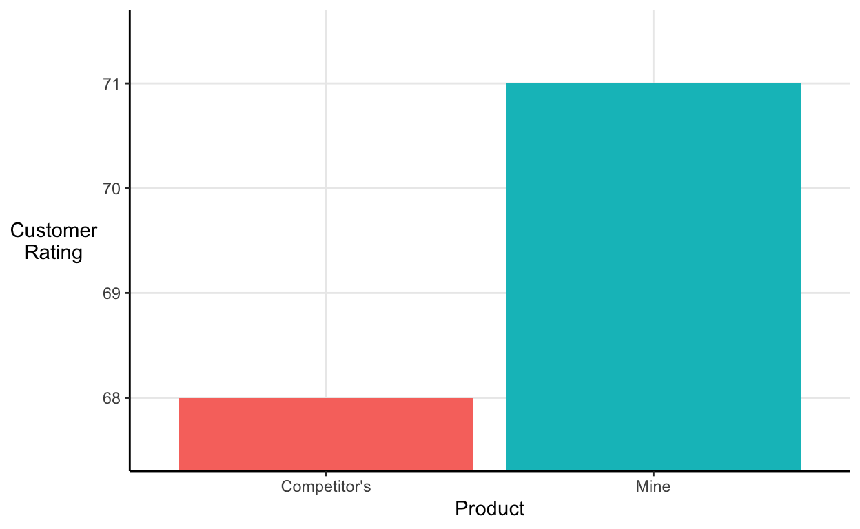
It looks like my product blows my competitor’s out of the water. However, notice where the y-axis starts and ends.
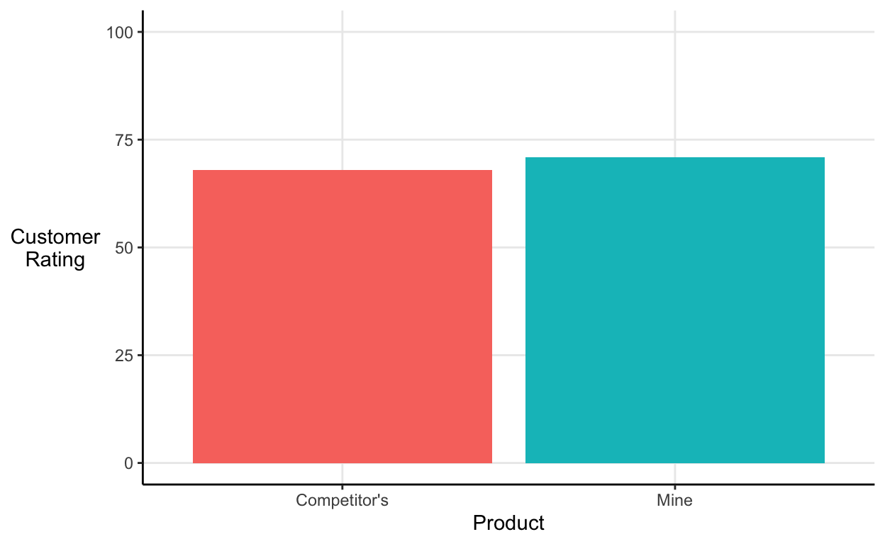
If we’re being strict, the y-axis should include the full range of values that customers were able to provide (it should at the very least include 0 if that’s a possible value). Once we properly format the graph my product looks a little less impressive:
Show code
# Bar chart with truncated y-axis
ggplot(product_ratings, aes(x = Product, y = mean_rating, fill = Product)) +
  geom_col() +
  scale_fill_discrete(guide = "none") +
  scale_y_continuous("Customer\nRating", limits = c(0, 100)) +
  theme_classic() +
  theme(axis.title.y = element_text(angle = 0, vjust = 0.5),
        panel.grid.major = element_line())
Discontinuous axes
Condensing a small portion of the x-axis can be used to falsely emphasise a few data points.
For example, say I’m selling security systems and I want to put a scary graph on the leaflet I drop through people’s letterboxes. I might include a line graph like this one that exaggerates the recent increase in the number of burglaries:
Show code
# Discontinuous line graph
tibble(Year = c("2009", "2010", "2011", "2012", "2013", "2014", "2019"),
       burglary_count = c(100, 102.5, 105, 107.5, 110, 112.5, 125)) %>%
  ggplot(aes(x = Year, y = burglary_count)) +
  geom_line(group = 1) +
  scale_y_continuous("Burglary\nCount") +
  theme_classic() +
  theme(axis.title.y = element_text(angle = 0, vjust = 0.5),
        panel.grid.major = element_line())
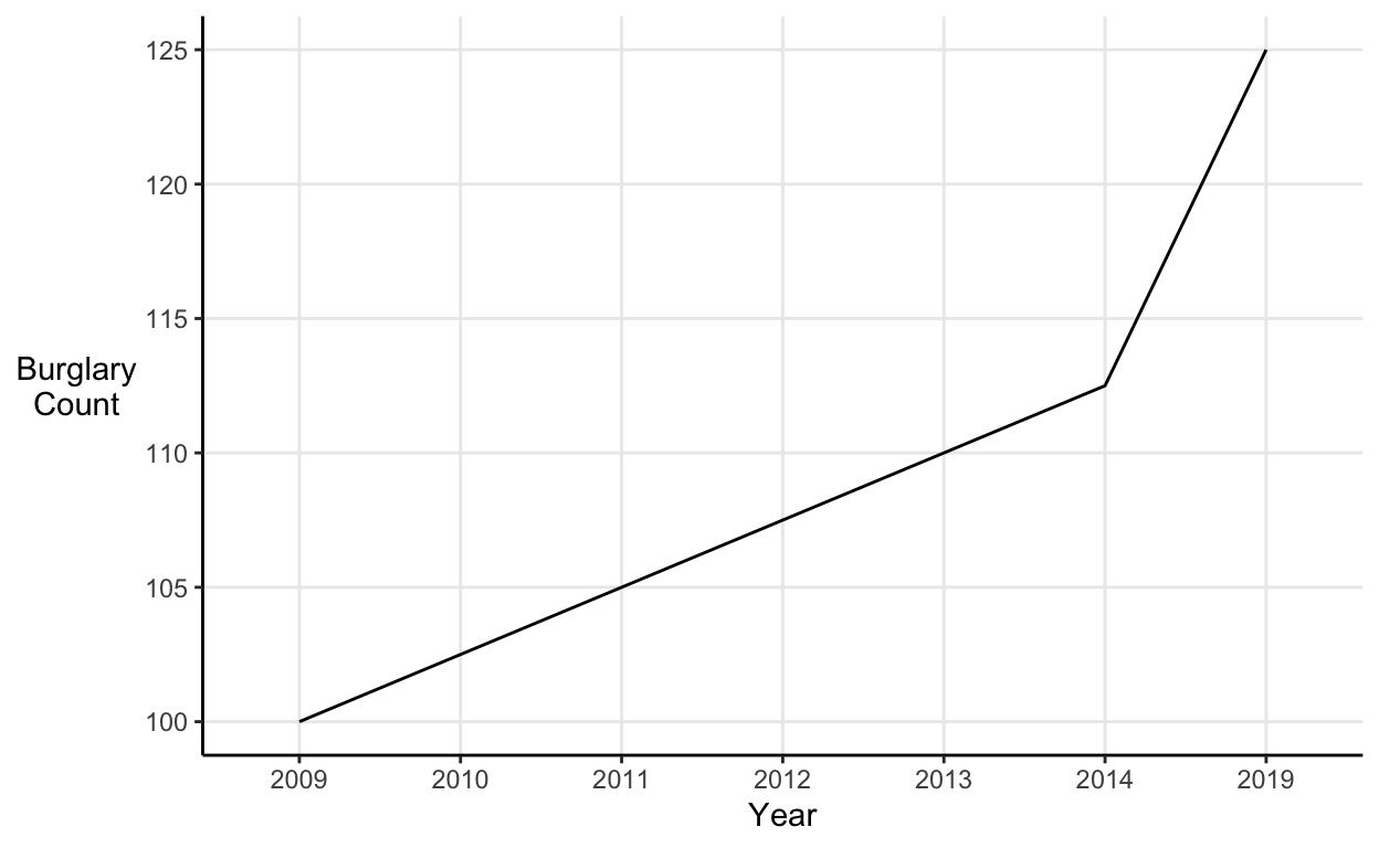
However, the apparent spike in burglaries is just a result of the fact that 5 years of increases have been squeezed into one notch on the x-axis.
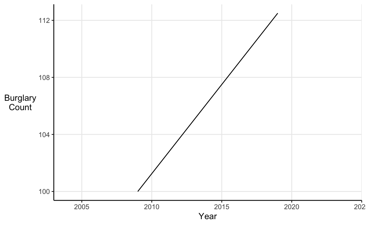
Elongated axes
Discontinuous axes make a change look more extreme by removing some values, but changes can also be exaggerated by elongating an axis using irrelevant blank values.
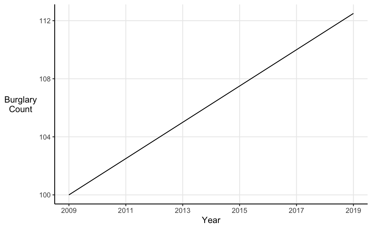
For example, take a similar line graph to the one discussed above. If we plot the graph without any trickery, then the data seem to show a steady increase in the number of burglaries:
Show code
# Regular x-axis line graph
tibble(Year = c(2009:2019), burglary_count = c(seq(100, 112.5, 1.25))) %>%
  ggplot(aes(x = Year, y = burglary_count)) +
  geom_line(group = 1) +
  scale_y_continuous("Burglary\nCount") +
  scale_x_continuous(breaks = c(2009, 2011, 2013, 2015, 2017, 2019)) +
  theme_classic() +
  theme(axis.title.y = element_text(angle = 0, vjust = 0.5),
        panel.grid.major = element_line())
However, we can make the same data look much more extreme by including space on the x-axis for years without any data. This narrows the visual space over which the same increase in our data must be plotted (meaning the line must be steeper). Thus, the same increase over the same timespan looks much more drastic:
Show code
# Elongated x-axis line graph
tibble(Year = c(2009:2019), burglary_count = c(seq(100, 112.5, 1.25))) %>%
  ggplot(aes(x = Year, y = burglary_count)) +
  geom_line(group = 1) +
  scale_y_continuous("Burglary\nCount") +
  coord_cartesian(xlim = c(2004, 2024)) +
  theme_classic() +
  theme(axis.title.y = element_text(angle = 0, vjust = 0.5),
        panel.grid.major = element_line())
Duplicate axes
Duplicating the y-axis allows you to tell any story you like with the data. If the two axes measure quantities in the same units then you can shift them without limit. A prominent example of this kind of manipulation is a graph presented by U.S. Representative Jason Chaffetz during a hearing on planned parenthood:
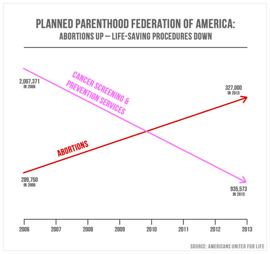
A good general rule is ‘when you want to use a double y-axis, use two graphs instead’. There are some instances when it’s defensible, I like a pareto chart as much as the next guy, if you’re using two different measures (i.e. different units) and only making ‘within-axis’ comparisons (rather than just shifting the left-hand y-axis up or down and to make your point).
If we plot Chaffetz’s chart properly it looks a little less like doctors are too busy with abortions to treat cancer:
Show code
# Correcting Chaffetz
tibble(Year = c(2006, 2013),
       Cancer = c(2007371, 935573),
       Abortions = c(289750, 327000)) %>%
  melt(id.vars = "Year") %>%
  ggplot(aes(x = Year, y = value, col = variable)) +
  geom_line(arrow = arrow(length = unit(0.15, "inches"), type = "closed")) +
  scale_y_continuous("Freq.", labels = scales::comma) +
  scale_x_continuous(breaks = c(2006:2013)) +
  scale_color_manual("Procedure\nPurpose",
                     values = c("Cancer" = "#FF96A7", "Abortions" = "red")) +
  theme_classic() +
  theme(axis.title.y = element_text(angle = 0, vjust = 0.5),
        panel.grid.major = element_line())
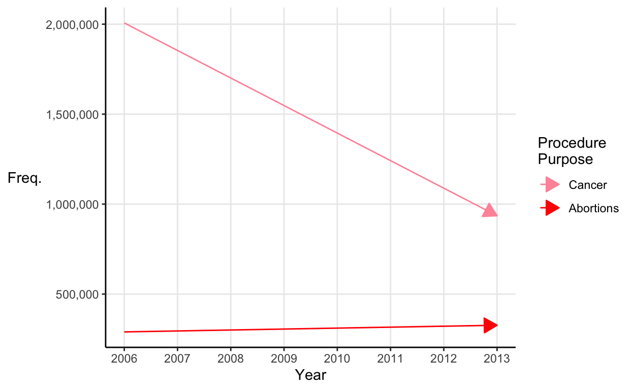
There are still problems with this graph (just plotting two time series and looking for a relationship is setting yourself up to over-interpret a spurious correlation) but it’s better than before.
Dodgy reporting
A few miscellaneous tactics that people use to fudge their reporting.
Hiding a decrease in the cumulative
Say you run a company where sales have decreased every quarter this year. You desperately need to show your board an impressive looking sales chart to quell their fears. Just hide the decrease in the cumulative total for the past few years (you’d be in good company):
Show code
# Cumulative sales line graph
ggplot(quarterly_sales, aes(x = quarter, y = cum_sales)) +
  geom_area() +
  scale_y_continuous("Sales\n(cumulative)") +
  scale_x_continuous("Quarter", expand = c(0.005, 0)) +
  theme_classic() +
  theme(axis.title.y = element_text(angle = 0, vjust = 0.5),
        panel.grid.major = element_line())
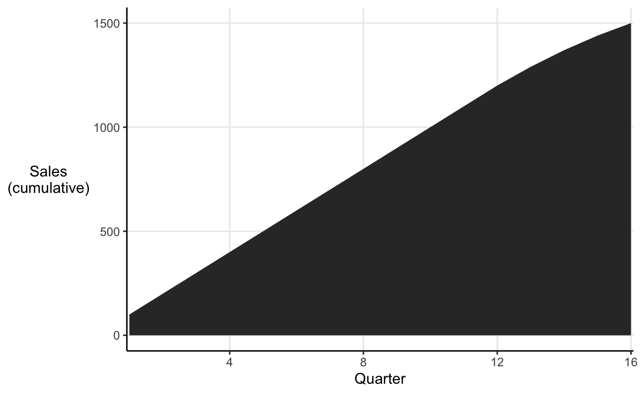
The decrease in the cumulative chart barely even registers, nothing to worry about here. The individual quarterly sales tell a slightly less rosy story:
Show code
# Quarterly sales bar chart
ggplot(quarterly_sales, aes(x = quarter, y = sales)) +
  geom_col() +
  scale_y_continuous("Sales") +
  labs(x = "Quarter") +
  theme_classic() +
  theme(axis.title.y = element_text(angle = 0, vjust = 0.5),
        panel.grid.major.y = element_line())
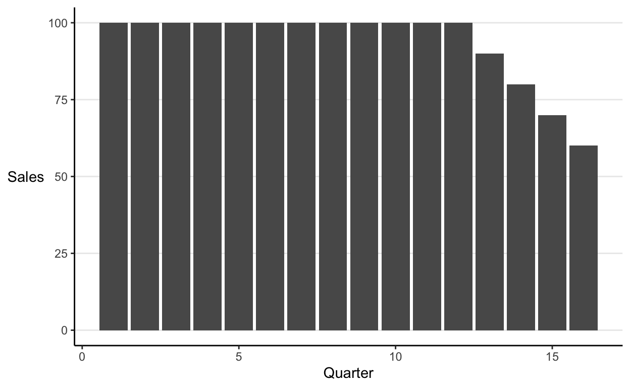
It’s now apparent that in the past quarter you sold 60% of the volume that you did in the same period last year.
Comparing apples and oranges
Amalgamating
The way data is grouped has an impact on the conclusions readers draw from it. One tactic to watch out for is when data has been binned into groups with unequal ranges.
For instance, say your parents were on your case about your latest maths test and you were so committed to deceiving them that you whipped up a histogram that showed your score of 75 pretty favourably:
Show code
# Histogram with favourable grouping
ggplot(maths_test, aes(x = score, fill = ..count..)) +
  geom_histogram(breaks = c(seq(10, 74, 4), 90)) +
  scale_y_continuous("Count") +
  scale_x_continuous("Score", breaks = c(0, 25, 50, 75)) +
  scale_fill_continuous(guide = "none") +
  theme_classic() +
  theme(axis.title.y = element_text(angle = 0, vjust = 0.5),
        panel.grid.major = element_line())
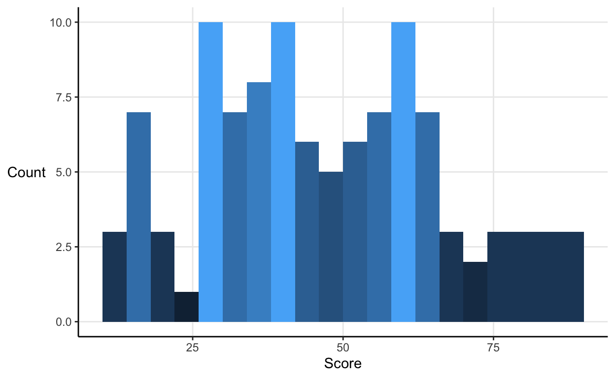
Your parents will be pleased that you’re in the group of your class’ very top scorers.
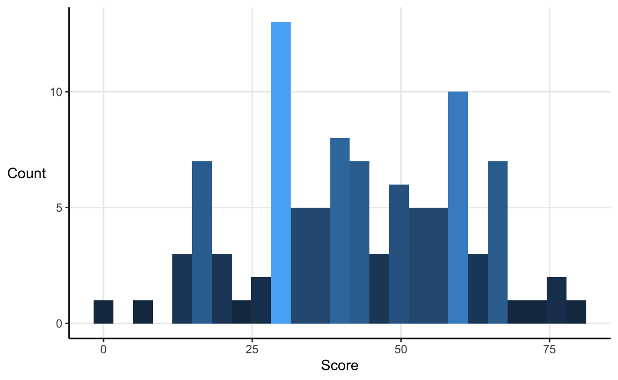
However, if we plot the same data with equal bin widths the little bit of fudging becomes apparent.
Show code
# Histogram with fair grouping
ggplot(maths_test, aes(x = score, fill = ..count..)) +
  geom_histogram(bins = 25) +
  scale_y_continuous("Count") +
  scale_x_continuous("Score", breaks = c(0, 25, 50, 75)) +
  scale_fill_continuous(guide = "none") +
  theme_classic() +
  theme(axis.title.y = element_text(angle = 0, vjust = 0.5),
        panel.grid.major = element_line())
If you’re writing your own reports then use equal bins widths, either in percentile or absolute terms. If you’re reading someone else’s, then make sure they do too.
Subdividing
Amalgamating involves people using suspect grouping decisions to make their point. Subdividing is the opposite. It involves misleadingly splitting the data until it implies what you want it to.
For instance, the U.S. CDC listed the top 2 causes of death in 2013 as:
- Heart disease = 611,105
- Cancer = 584,881
But, both of these are actually groups of conditions. So, say you’re trying to get more funding for cancer research you might subdivide the heart disease category but not the cancer one. Then you could, honestly but misleadingly, report that the top causes of death were:
- Cancer = 584,881
- Acute myocardial infarction = 116,793
- Heart failure = 65,120
- Hypertensive heart disease = 37,144
- Acute rheumatic fever and chronic rheumatic heart disease = 3,260
So, be on the look out for suspicious subdividing.
Conclusion
Levitin provides a solid compilation of mistakes to avoid and tricks to look out for when producing and reading research respectively. However, given his background in psychology and neuroscience, I was hoping for a more general thread pulling the examples together concerning why the human brain is ‘fooled’ by particular ways of presenting information rather than just what those presentations are.