I was given Infinite Powers by Steven Strogatz as a Christmas present (thanks Grandma). It’s a good book and I’d recommend it to anyone who ever sat in a maths class and genuinely asked the teacher, “err, but, like, why?” Most of the time, in my experience anyway, questions like that one didn’t get a good answer. The response tended to be either a ‘why must you always interrupt me’ look or an exasperated “because it’s on the mark scheme and you need to know this for the exam”.
One of my favourite sections of the book involved Strogatz recounting how Archimedes estimated the value of \(\pi\). The reason being that there’s a popular data science interview question which also requires the applicant to estimate \(\pi\). So, I thought it would be fun to compare Archimedes’ estimate to what I’ll be (shamelessly and repeatedly) calling Rchimedes’ estimate.
Archimedes’ estimate
\(\pi\) is defined as the ratio between the circumference and diameter of a circle
\[\pi = \frac{C}{d}\]
We know that the diameter is twice the radius:
\[d = 2r\]
Which means we can write:
\[\pi = \frac{C}{2r}\]
If we approximate the circumference of a circle using a hexagon inside it (as shown in the image below), then we know that (because a hexagon is 6 equilateral triangles) the distance around the edge of the hexagon (in bold) is \(6r\).

Since the hexagon is inside the circle, we know that the distance around its edges must be an underestimate of the circumference. So, we can write:
\[C > 6r\]
If we substitute this into our previous formula for \(\pi\) we get:
\[\pi = \frac{C}{2r} > \frac{6r}{2r} = 3\]
In other words, we get a lower bound for the true value of \(\pi\). We know it must be larger than 3.
Now we can carry out the same process with a hexagon that is just outside the circle to get an upper bound for \(\pi\).
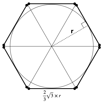
Whereas before each edge in the hexagon was length \(r\), now each edge has length \(\frac{2}{3}\sqrt{3}\times r\) (you can figure this out from the fact that the height of each of the equilateral triangles comprising the hexagon is \(r\)). So, we can multiply this by 6 to find the distance around the edge of the external hexagon:
\[6 \times \frac{2}{3}\sqrt{3}\times r = 4r\sqrt{3}\]
This time we know that our hexagon is an overestimate for the circumference:
\[C < 4r\sqrt{3}\]
If we again substitute this into our formula for \(\pi\) we get:
\[\pi = \frac{C}{2r} < \frac{4r\sqrt{3}}{2r} = 2\sqrt{3}\]
Now we have a corresponding upper bound for the true value of \(\pi\). We know it must be less than \(2\sqrt{3}\), which rounded to 2 decimal places is \(3.46\).
So, using our two hexagons we have found an interval for \(\pi\):
\[3 < \pi < 3.46\]
Staggeringly, Archimedes carried out a process equivalent to the one we just played through with a 96-sided shape and found the following interval:
\[3\frac{10}{71} < \pi < 3\frac{10}{70}\] Which rounded to 3 decimal places is:
\[3.141 < \pi < 3.143\]
This means he found \(\pi\) correct to 2 decimal places, \(3.14\), which is as much precision as most people know \(\pi\) to nowadays.
Rchimedes’ estimate
OK, you’re dressed to impress, you’ve politely said yes to a tea because you read a social psychology paper once that said interviewers preferred candidates that did, and you can feel a few beads of nervous sweat on the small of your back. You sit down at the interview table and the interviewer hands you a laptop with a set of instructions already open:
You have a function which takes the input \(n\) and outputs \(n\) random numbers between 0 and 1. Estimate the value of \(\pi\).
After the customary moment of panic, you decide to actually think it through.
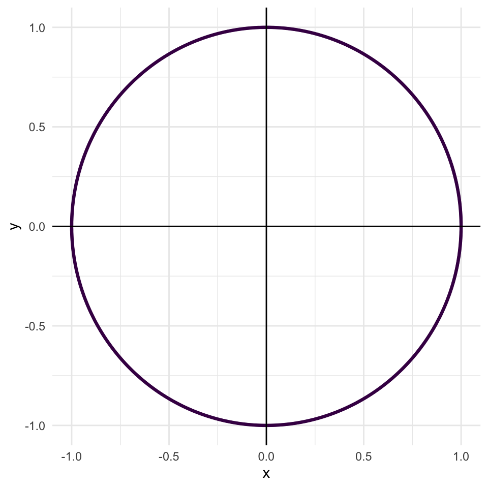
Well, the easiest way you can think of to estimate \(\pi\) is to find the area of a circle with a radius of \(1\).
After all,
\[\begin{aligned} \text{Area of a circle} &= \pi \times \text{radius}^2 \\ \end{aligned}\]
So if \(\text{radius} = 1\), then
\[\begin{aligned} \text{Area of a circle} &= \pi \times 1^2 \\ &= \pi \end{aligned}\]
Alright, so what would a circle with radius of 1 look like?
Show code
circle_coords <- function(center = c(0, 0), radius = 1, n_points = 1000) {
    centre_angle <- seq(0, 2*pi, length.out = n_points)
    x_coord <- center[1] + radius * cos(centre_angle)
    y_coord <- center[2] + radius * sin(centre_angle)
    tibble(x = x_coord, y = y_coord)
}

r_1 <- circle_coords()

r_1 %>%
  ggplot(aes(x = x, y = y)) +
  geom_point(size = 0.5, col = "#440154FF") +
  geom_vline(aes(xintercept = 0)) +
  geom_hline(aes(yintercept = 0)) +
  theme_minimal()
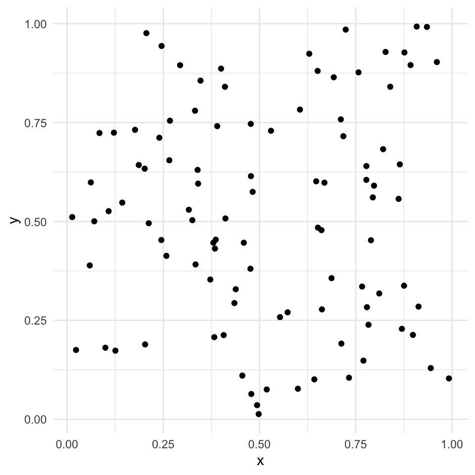
How does this help us? Well, if we use the random number function twice we can generate pairs of random coordinates. Let’s plot 100 such coordinates:
Show code
random_xy %>%
  ggplot(aes(x = x, y = y)) +
  geom_point() +
  theme_minimal()
Now, if we superimpose our random pairs of coordinates onto our circle with radius 1:
Show code
r_1 %>%
  ggplot(aes(x = x, y = y)) +
  geom_point(size = 0.5, col = "#440154FF") +
  geom_point(data = random_xy, aes(x = x, y = y)) +
  geom_vline(aes(xintercept = 0)) +
  geom_hline(aes(yintercept = 0)) +
  theme_minimal()
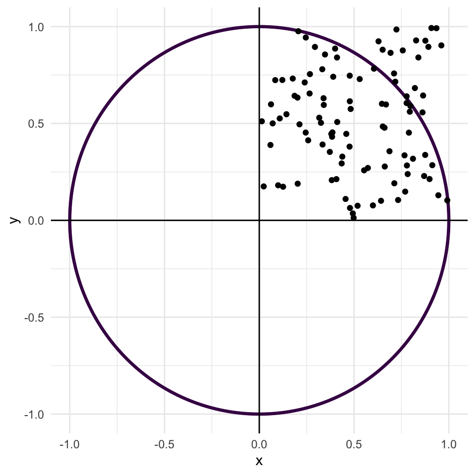
Hopefully the plan is starting to become clear.
We need to calculate the proportion of random points that are inside the circle.
Show code
r_1 %>%
  ggplot(aes(x = x, y = y)) +
  geom_point(size = 0.5, col = "#440154FF") +
  geom_point(data = random_xy, aes(x = x, y = y, col = in_circle)) +
  geom_vline(aes(xintercept = 0)) +
  geom_hline(aes(yintercept = 0)) +
  scale_color_manual(guide = "none",
                     values = c("#31688EFF", "#FDE725FF")) +
  theme_minimal()
Show code
prop_inside <- mean(random_xy$in_circle)
pi_estimate <- 4*prop_inside
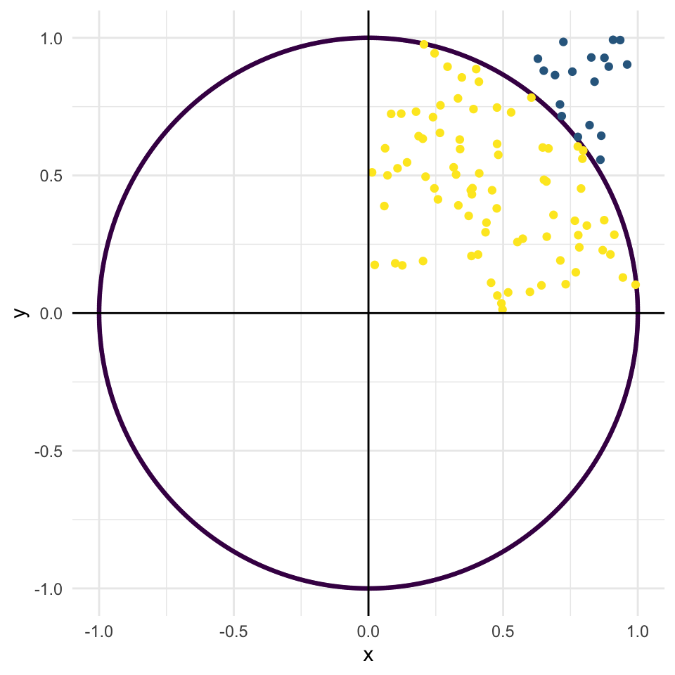
In this instance, the proportion of our random points that fall inside the circle is 0.82. This is an estimate for the area of one quarter of the circle.
So, to find an estimate for the area of the whole circle (which we know to be \(\pi\)) all we have to do is multiply that proportion by 4. In this case, our estimate for \(\pi\) turns out to be 3.28.
That’s an OK estimate but, what if we want a greater degree of accuracy? All we need to do is use more random points.
Say we ran through the whole process again but this time with 1000 points:
Show code
set.seed(1)
random_xy <- tibble(x = runif(1000), y = runif(1000)) %>%
  mutate(o_dist = sqrt(x^2 + y^2),
         in_circle = if_else(o_dist <= 1, T, F))

r_1 %>%
  ggplot(aes(x = x, y = y)) +
  geom_point(size = 0.5, col = "#440154FF") +
  geom_point(data = random_xy, aes(x = x, y = y, col = in_circle)) +
  geom_vline(aes(xintercept = 0)) +
  geom_hline(aes(yintercept = 0)) +
  scale_color_manual(guide = "none",
                     values = c("#31688EFF", "#FDE725FF")) +
  theme_minimal()
Show code
prop_inside <- mean(random_xy$in_circle)
pi_estimate <- 4*prop_inside
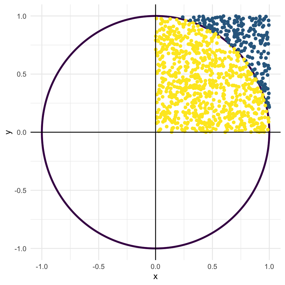
Now, the proportion of points inside the circle is 0.787 giving us an
estimate for \(\pi\) of 3.148.
R provides the value of \(\pi\) to 6 decimal places as 3.141593.
We’re getting closer.
Can we beat a guy who’s been dead for over 2000 years?
So we’ve got a process that can help us estimate \(\pi\). We overlay random points on one quarter of a circle, find out the proportion that fall inside the circle, and then multiply by 4.
Here’s an R function that plays through this process for us:
Show code
R_chimedes <- function(n_points) {
  # Generate random pair of coordinates between 0 and 1
  x <- runif(n_points)
  y <- runif(n_points)
  # For each pair find distance from the origin
  o_dist <- sqrt(x^2 + y^2)
  # If o_dist <= 1, then inside or on the circle
  in_or_out <- o_dist <= 1
  # Estimate pi
  4 * mean(in_or_out == TRUE)
}
All we need to do is choose how many random points to use,
n_points.
So, how many random points do we need before we are more accurate than Archimedes was?
Let’s try a few different powers of 10. For each different value of
n_points, we’ll calculate 3 estimates of \(\pi\).
Show code
set.seed(1)
estimates <- tibble(n_points = 10^(2:8),
                    attempt_1 = map_dbl(n_points, R_chimedes),
                    attempt_2 = map_dbl(n_points, R_chimedes),
                    attempt_3 = map_dbl(n_points, R_chimedes)) %>%
  pivot_longer(cols = -n_points, names_to = "Estimate") %>%
  mutate(pi_6dp = pi,
         archimedes_low = 3 + 10/71,
         archimedes_high = 3 + 10/70)
Show code
estimates %>%
  ggplot(aes(x = n_points, y = value)) +
  geom_ribbon(aes(ymin = archimedes_low, ymax = archimedes_high),
              fill = "#440154FF",
              alpha = 0.2) +
  geom_line(aes(y = pi_6dp), col = "#440154FF", lty = 2) +
  geom_point(aes(shape = Estimate, col = Estimate), size = 1.5) +
  scale_x_log10("No. of random points",
                breaks = 10^(2:8),
                labels = trans_format("log10", math_format(10^.x))) +
  scale_y_continuous("Value") +
  scale_color_manual(values = c("#31688EFF", "#35B779FF", "#FDE725FF")) +
  labs(caption = "The dashed purple line is pi to 6 dp.\nPurple band is Archimedes' range.") +
  theme_minimal() +
  theme(axis.title.y = element_text(angle = 0, vjust = 0.5))
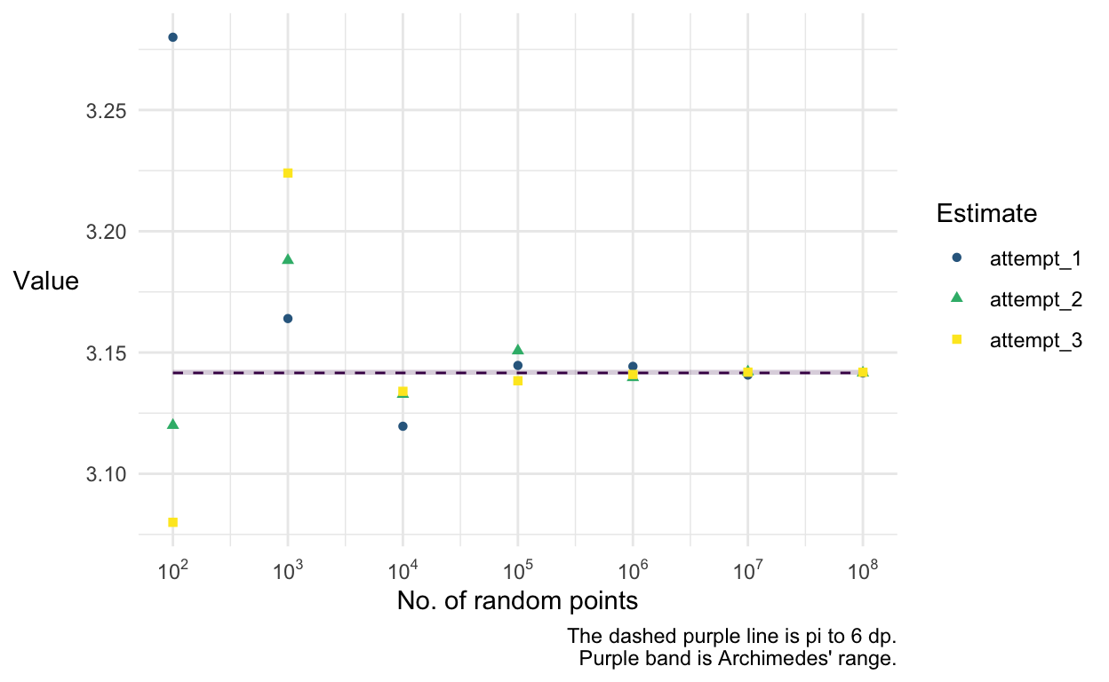
We can see that once we use \(1,000,000\) (\(10^6\)) random points, our estimate is getting pretty close consistently. The graph gets too small to read so let’s zoom in on the right hand end of the x-axis:
Show code
estimates %>%
  ggplot(aes(x = n_points, y = value)) +
  geom_ribbon(aes(ymin = archimedes_low, ymax = archimedes_high),
              fill = "#440154FF",
              alpha = 0.2) +
  geom_line(aes(y = pi_6dp), col = "#440154FF", lty = 2) +
  geom_point(aes(shape = Estimate, col = Estimate), size = 1.5) +
  scale_x_log10("No. of random points",
                breaks = 10^(6:8),
                labels = trans_format("log10", math_format(10^.x)),
                limits = c(10^6, 10^8)) +
  scale_y_continuous("Value", limits = c(3.139, 3.145)) +
  scale_color_manual(values = c("#31688EFF", "#35B779FF", "#FDE725FF")) +
  labs(caption = "The dashed purple line is pi to 6 dp.\nPurple band is Archimedes' range.") +
  theme_minimal() +
  theme(axis.title.y = element_text(angle = 0, vjust = 0.5))
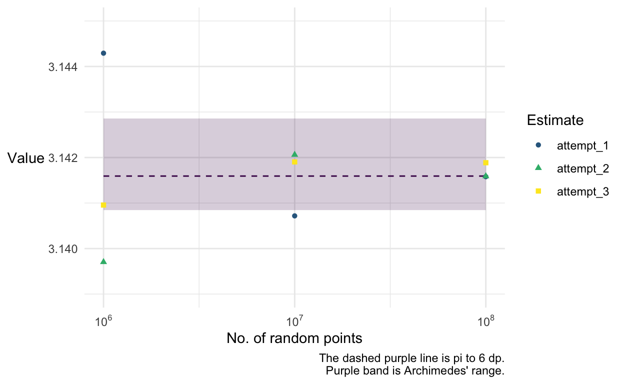
Now we can see that (in this instance) when we use \(100,000,000\) random points all 3 of our estimates for \(\pi\) are more accurate than the range Archimedes specified. This blew me away and I think it compounds just how impressive his calculation was.
Knowing vs. Understanding
The thought that I kept returning to whilst reading Infinite Powers was that there is a much bigger difference than I had realised between knowing something and understanding it. For example, I have known for a long time that the formula for the area of a circle was \(\pi r^2\) but until reading this book I didn’t have any sense of understanding about why that was true.
Throughout all of school and most of uni all I really did was know stuff. Now I want to understand stuff. And, if that means that there’s necessarily less stuff involved, then I’m fine with that.