Introduction
Someone recently pointed me in the direction of this paper by David Arthur and Sergei Vassilvitskii, k-means++: The Advantages of Careful Seeding. I can’t claim to understand the proofs but their key idea is quite intuitive.
What is the k-means problem?
We are given an integer \(k\) and a set of \(n\) data points.
We wish to choose \(k\) centers, \(C\), so as to minimise the “potential function”:
\[\phi = \sum \text{min} ||x - c||^2\]
- For each center, we set one cluster to be the set of data points that are closer to that center than to any other.
The k-means algorithm
Simple and fast algorithm that attempts to locally improve an arbitrary k-means clustering.
Steps:
- Arbitrarily choose \(k\) initial centers \(C= \{c_1, ..., c_k\}\)
- For each \(i \in \{1, ..., k\}\), set the cluster \(C_i\) to be the set of points that are closer to \(c_i\) than they are to \(c_j\) for all \(j \ne i\).
- For each \(i \in \{1, ..., k\}\), set \(c_i\) to be the centre of mass of all points in \(C_i\).
\[c_i = \frac{1}{|C_i|} \sum_{x \in C_i} x\]
- Note that \(|C_i|\) is the cardinality operator. It returns the number of elements in the set.
- Repeat steps 2 and 3 until \(C\) no longer changes.
Standard practice is to choose the initial centres uniformly at random from \(X\).
For Step 2, ties may be broken arbitrarily as long as the method is consistent.
Algorithm is only guaranteed to find a local optimum, which can sometimes be quite poor.
The k-means++ algorithm
Arthur and Vassilvitskii propose a specific way of choosing the initial set of cluster centers.
Let \(D(x)\) denote the shortest distance from a data point \(x\) to the closest centre we have already chosen.
1.a. Choose an initial center \(c_1\) uniformly at random \(X\).
1.b. Choose the next center \(c_i\), selecting \(c_i = x'\) with probability \(\frac{D(x')^2}{\sum D(x)^2}\).
- They call this “\(D^2\) weighting”
1.c. Repeat Step 1b. until we have chosen \(k\) centres.
2 - 4. Proceed with standard k-means algorithm.
Explore by manually clustering in one dimension
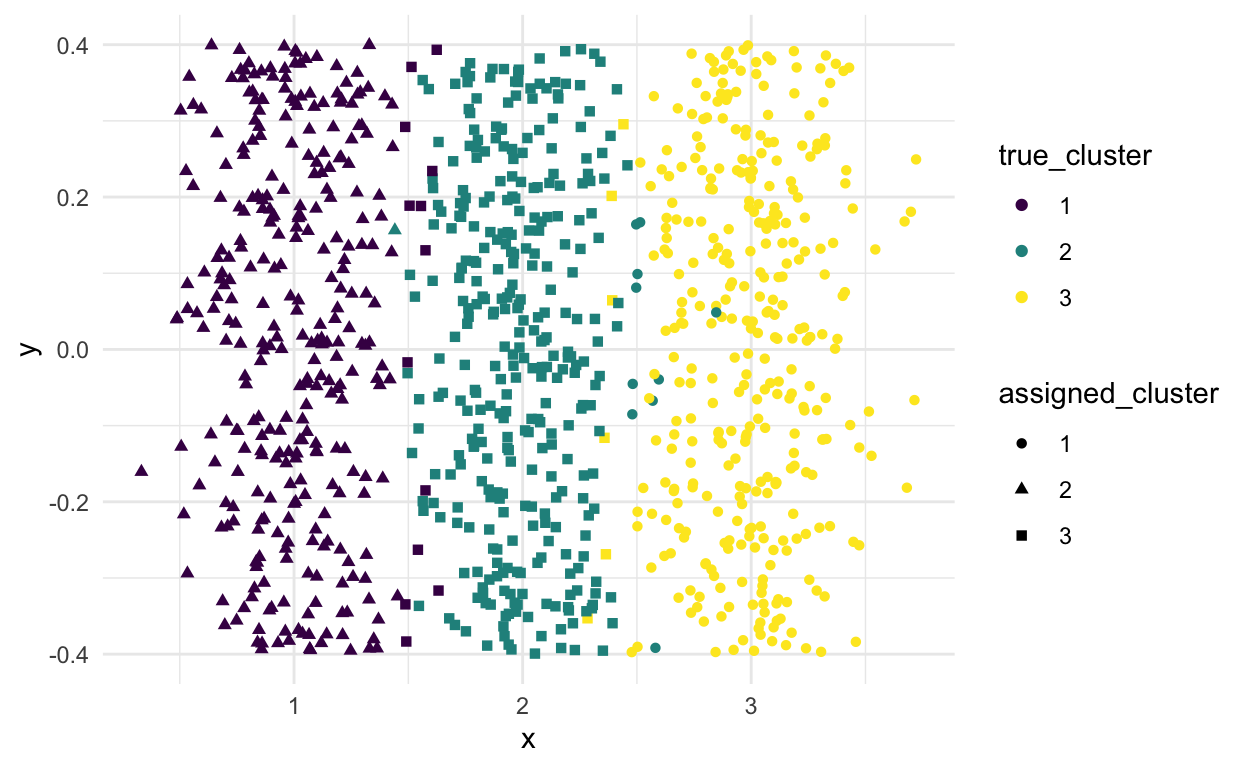
Using k-means
Show code
kmeans_clusters <- kmeans(X, centers = 3)

tibble(x = X,
       true_cluster = factor(true_cluster),
       assigned_cluster = factor(kmeans_clusters$cluster)) %>%
  ggplot(aes(x = x, y = 0, color = true_cluster, shape = assigned_cluster)) +
  geom_jitter() +
  scale_color_viridis_d()
Using k-means++
Say that we set \(k = 3\)
Show code
[1] 1Show code
# Find the 2nd center
c_2 <- second_centre %>%
  sample_n(size = 1, weight = prob) %>%
  pull(x)

# Find probability for all other points of being the next centre
third_centre <- second_centre %>%
  rename(d_1 = d) %>%
  mutate(d_2 = x - c_2) %>%
  rowwise() %>%
  mutate(d_min = min(abs(d_1), abs(d_2))) %>%
  ungroup() %>%
  mutate(d_squared = d_min^2,
         d_squared_sum = sum(d_squared),
         prob = d_squared/d_squared_sum)

sum(third_centre$prob)
[1] 1Show code
# Find the next center
c_3 <- third_centre %>%
  sample_n(size = 1, weight = prob) %>%
  pull(x)

# Run the usual k-means algorithm using the 3 centres we've selected
kmeans_pp_clusters <- kmeans(x = X, centers = c(c_1, c_2, c_3))

tibble(x = X,
       true_cluster = factor(true_cluster),
       assigned_cluster = factor(kmeans_pp_clusters$cluster)) %>%
  ggplot(aes(x = x, y = 0, color = true_cluster, shape = assigned_cluster)) +
  geom_jitter() +
  scale_color_viridis_d()
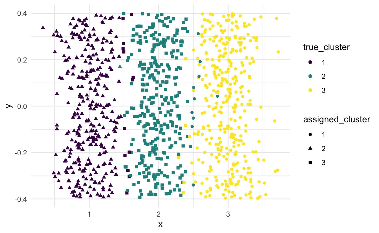
- Not sure it makes much difference in this case but the paper says you’ll get better results in general.