Introduction
I’m a little bit scared general AI is gonna kill us all. So I picked up The Alignment Problem by Brian Christian hoping that he would quell my fears. Sadly, he didn’t. But he did succeed in distracting me for a little while with his second chapter on Fairness which highlighted issues of bias in the application of narrow machine learning techniques. So, to continue that blissful distraction, I wanted to explore one of the papers he cited, Inherent Trade-Offs in the Fair Determination of Risk Scores by Kleinberg et al.
Different meanings of “fair”
The paper starts by formalising 3 common notions of fairness.
If we think about making predictions about a population of people composed of two groups, then we can talk about fairness in terms of:
Calibration: If we predict that X% of people will experience an event, then for both group A and group B in our population X% of the people do experience the event.
Balance for the negative class: The average score assigned to people of group A who belong to the negative class (do not experience the event) should be the same as the average score assigned to people of group B who belong to the negative class.
Balance for the positive class: The average score assigned to people of group A who belong to the positive class (do experience the event) should be the same as the average score assigned to people of group B who belong to the positive class.
An illustrative example
This example is adapted from from the Econ-ML blog and re-written in R.
Imagine we’re training a supervised learning model to predict whether a person has a disease. There are two groups, A and B, in our population that we want to treat ‘fairly’.
Let’s also say that Group A and Group B have different average probabilities of getting the disease.
- The mean probability for Group A is 0.5
- The mean probability for Group B is 0.7
Let’s pretend our model is brilliant and predicts each individual’s true probability of having the disease. To apply these predictions, we might put people into different risk ‘buckets’ that are treated differently. For example, people in the higher risk buckets might be referred to specialists.
Show code
# Say that ML algorithm predicts the true probability
fake_ml <- tibble(group = c(rep("A", n_people), rep("B", n_people)),
                  true_probs = c(a_probs, b_probs)) %>%
  mutate(uniform_draw = runif(n = nrow(.), min = 0, max = 1),
         has_disease = uniform_draw < true_probs,
         ml_prediction = true_probs,
         ml_score = round(ml_prediction, digits = 1))
So, we know our model is accurate (because we faked the data to make it so). But, is it fair?
Is our model calibrated?
We can check the calibration of our model by looking within each bucket and seeing what proportion of people actually had the disease.
If we look within our “10% risk” bucket and find that roughly 10% of people had the disease, then our model is well calibrated.
If this is true for both groups in our population, then our model is fair with respect to calibration. This means that a score of “10% risk” means the same thing regardless of which group you belong to.
Show code
# Calibration
# - E.g. Do 10% of the people we put in the 10% category get the disease?
check_calibration <- fake_ml %>%
  group_by(group, ml_score) %>%
  summarise(prop_has_disease = mean(has_disease)) %>%
  mutate(across(c(ml_score, prop_has_disease),
                ~round(.x *100)))

check_calibration %>%
  ggplot(aes(x = ml_score, y = prop_has_disease, fill = group)) +
  geom_col(position = "dodge") +
  geom_abline(slope = 1, intercept = 0, linetype = 2) +
  scale_x_continuous("Bucketed risk score given by ML algorithm",
                     n.breaks = 10) +
  scale_y_continuous("Percentage of\npeople with\nthe disease",
                     n.breaks = 10) +
  scale_fill_viridis_d("Group") +
  labs(caption = "Dashed line represents perfect calibration")
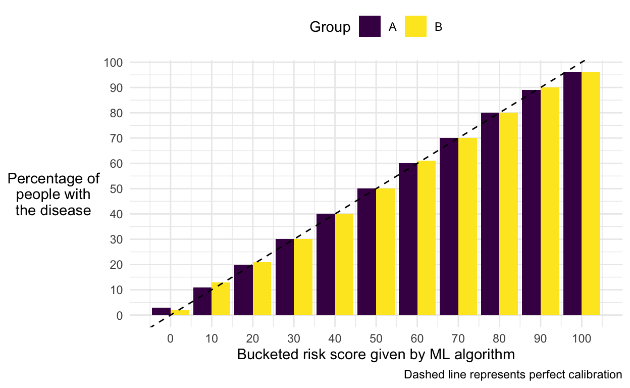
We can see that our model is calibrated equally well for both groups.
Is our model balanced?
But, is our model balanced with respect to the positive class? In other words, do people with the disease in the 2 groups have the same average score?
Show code
| group | mean_score |
|---|---|
| A | 0.5867175 |
| B | 0.7442754 |
No. People in group B have a higher average score.
How about the opposite problem? Is our model balanced with respect to the negative class? In other words, do people without the disease in the 2 groups have the same average score?
Show code
| group | mean_score |
|---|---|
| A | 0.4129972 |
| B | 0.5862818 |
No. Again, people in group B have a higher average score.
So what?
Ok, so we’ve found that our model isn’t fair with respect to balance. But, what difference does this make practically?
A key problem is that it means we’ll make different types of errors in our predictions about people in the two groups.
Imagine that instead of putting our model’s predictions into 10 buckets, we used them to decide whether to offer treatment. Say we offered treatment to anyone who our model predicts has a risk of greater than 0.5.
We can then look at the types of errors we would make:
Show code
binary_treatment <- fake_ml %>%
  mutate(is_treated = ml_prediction > 0.5) %>%
  group_by(group, has_disease, is_treated) %>%
  summarise(n = n(), .groups = "drop") %>%
  group_by(group) %>%
  mutate(prop_of_group = round(n/sum(n), 2)) %>%
  ungroup() %>%
  mutate(correct = has_disease == is_treated,
         direction = if_else(is_treated == TRUE, "positive", "negative"),
         outcome = str_to_title(paste(correct, direction)))

# Extract individual numbers for text
a_tp <- binary_treatment %>%
  filter(group == "A" & outcome == "True Positive") %>%
  pull(prop_of_group)

a_tn <- binary_treatment %>%
  filter(group == "A" & outcome == "True Negative") %>%
  pull(prop_of_group)

a_fp <- binary_treatment %>%
  filter(group == "A" & outcome == "False Positive") %>%
  pull(prop_of_group)

a_fn <- binary_treatment %>%
  filter(group == "A" & outcome == "False Negative") %>%
  pull(prop_of_group)

b_tp <- binary_treatment %>%
  filter(group == "B" & outcome == "True Positive") %>%
  pull(prop_of_group)

b_tn <- binary_treatment %>%
  filter(group == "B" & outcome == "True Negative") %>%
  pull(prop_of_group)

b_fp <- binary_treatment %>%
  filter(group == "B" & outcome == "False Positive") %>%
  pull(prop_of_group)

b_fn <- binary_treatment %>%
  filter(group == "B" & outcome == "False Negative") %>%
  pull(prop_of_group)

binary_treatment %>%
  select(Group = group, outcome, prop_of_group) %>%
  pivot_wider(names_from = outcome, values_from = prop_of_group) %>%
  kable()
| Group | True Negative | False Positive | False Negative | True Positive |
|---|---|---|---|---|
| A | 0.34 | 0.16 | 0.16 | 0.34 |
| B | 0.10 | 0.20 | 0.06 | 0.64 |
We can see that the overall accuracy is the two groups is fairly similar:
- In Group A:
- 0.34 + 0.34 = 0.68 accuracy
- In Group B:
- 0.64 + 0.1 = 0.74 accuracy
However, we can also see that false positives are more common for Group B and that false negatives are more common for Group A.
- A false positive would mean we treated someone for the disease who didn’t have it.
- A false negative would mean that we didn’t treat someone for the disease who did have it.
We can imagine how these different types of errors might be deemed unfair. If you were in Group B, then you’d be more likely to have unnecessary treatment. Meanwhile, if you were in Group A, then you’d be more likely to miss out on necessary treatment.
Can we eat our cake and have it too?
The good news is that there are two scenarios when we can have both calibration and balance. The bad news is that both scenarios seem pretty unlikely. They are:
- When we have perfect predictions
- When we equal base rates across groups
To see why, let:
- \(N_t\) be the number of people in group \(t\)
- \(\mu_t\) be the number of people in group \(t\) who belong to the positive class
- \(x\) be the average score given to a member of the negative class
- \(y\) be the average score given to a member of the positive class
First, consider a single bin \(b\).
- If the calibration condition is met, then the expected total score given to the group-\(t\) people in bin \(b\) is equal to the expected number of group-\(t\) people in bin \(b\) who belong to the positive class.
- Summing over all bins, we find that the total score given to all people in group \(t\) (that is, the sum of the scores received by everyone in group t) is equal to the total number of people in the positive class in group \(t\), which is \(\mu_t\).
Second, consider the values of \(x\) and \(y\).
- If the balance condition is met for the negative and positive classes, then the values of \(x\) and \(y\) are the same for both groups.
We’ve now got five values that we can use to write down the total score for each group:
- The total number of people, \(N_t\).
- The average score given to a member of the negative class, \(x\).
- The average score given to a member of the positive class, \(y\).
- The total number of people in the positive class in group \(t\), \(\mu_t\).
- The total score given out to people in group \(t\), also \(\mu_t\).
\[\mu_t = (N_t − \mu_t)x + \mu_ty\]
Expressing the same thing verbally, we can say:
\[ \begin{aligned} \text{The total score given out to people in group}\;t &= (\text{The number of people in the negative class in group}\;t \\ &\times \text{The average score given to a member of the negative class}) \\ &+ (\text{The number of people in the positive class in group}\;t \\ &\times \text{The average score given to a member of the positive class}) \end{aligned} \]
This defines a line for each group \(t\) as a function of the two variables \(x\) and \(y\).
- This gives us a system of two linear equations (one for each group) in the unknowns \(x\) and \(y\).
\[ \begin{aligned} \mu_1 &= (N_1 − \mu_1)x + \mu_1y \;\;\;\;\;\;\;\;\;\;\;(1)\\ \mu_2 &= (N_2 − \mu_2)x + \mu_2y \;\;\;\;\;\;\;\;\;\;\;(2) \end{aligned} \]
If all three conditions — calibration, and balance for the two classes — are to be satisfied, then we must be at a set of parameters that represents a solution to the system of two equations.
One solution occurs when the base rates for the two groups are equal:
\[ \begin{aligned} \text{Re-arrange eq. (1)} \\ \mu_1 &= (N_1 − \mu_1)x + \mu_1y \\ \mu_1y &= \mu_1 - (N_1 − \mu_1)x \\ y &= 1 - \frac{(N_1 − \mu_1)x}{\mu_1} \\ \text{Substitute back into eq. (2)} \\ \mu_2 &= (N_2 − \mu_2)x + \mu_2y \\ \mu_2 &= (N_2 − \mu_2)x + \mu_2(1 - \frac{(N_1 − \mu_1)x}{\mu_1}) \\ \mu_2 &= N_2x − \mu_2x + \mu_2 - \frac{\mu_2(N_1 − \mu_1)x}{\mu_1} \\ 0 &= N_2x − \mu_2x - \frac{\mu_2(N_1 − \mu_1)x}{\mu_1} \\ 0 &= \mu_1N_2x − \mu_1\mu_2x - \mu_2x(N_1 − \mu_1) \\ 0 &= \mu_1N_2x − \mu_1\mu_2x +\mu_1\mu_2x - \mu_2N_1x \\ 0 &= \mu_1N_2x - \mu_2N_1x \\ \mu_2N_1x &= \mu_1N_2x \\ \frac{\mu_2}{N_2} &= \frac{\mu_1}{N_1} \\ \end{aligned} \]
- This means that the same proportion of people are in the positive
class in both groups
- I.e. We have equal base rates.
- In this case, the system of equations is satisfied by any choice of \(x\) and \(y\).
Another solution occurs when we have perfect predictions:
\[ \begin{aligned} \text{Re-arrange eq. (1)} \\ \mu_1 &= (N_1 − \mu_1)x + \mu_1y \\ \mu_1y &= \mu_1 - (N_1 − \mu_1)x \\ y &= 1 - \frac{(N_1 − \mu_1)x}{\mu_1} \;\;\;\;\;\;\;\;\;\;\;(3)\\ \text{Re-arrange eq. (2)} \\ \mu_2 &= (N_2 − \mu_2)x + \mu_2y \\ \mu_2y &= \mu_2 - (N_2 − \mu_2)x \\ y &= 1 - \frac{(N_2 − \mu_2)x}{\mu_2} \\ \text{Set equal to one another} \\ 1 - \frac{(N_1 − \mu_1)x}{\mu_1} &= 1 - \frac{(N_2 − \mu_2)x}{\mu_2} \\ \frac{(N_1 − \mu_1)x}{\mu_1} &= \frac{(N_2 − \mu_2)x}{\mu_2} \\ \mu_2(N_1 − \mu_1)x &= \mu_1(N_2 − \mu_2)x \\ \mu_2N_1x − \mu_1x &= \mu_1N_2x − \mu_2x \\ 0 &= \mu_1N_1x - \mu_2N_2x − \mu_2x + \mu_1x\\ 0 &= x(\mu_1N_1 - \mu_2N_2 − \mu_2 + \mu_1)\\ x &= 0\\ \text{Substitute back into eq. (3)} \\ y &= 1 - \frac{(N_1 − \mu_1) \times 0}{\mu_1} \\ y &= 1 \end{aligned} \]
- In this case we have \(x = 0\) and
\(y = 1\).
- I.e. An average score of 0 for members of the negative class
- I.e. An average score of 1 for members of the positive class
- This implies perfect predictions are made.
And so we arrive at the unsettling conclusion of Kleinberg et al’s paper:
Thus, the three conditions [calibration, positive balance, and negative balance] can be simultaneously satisfied if and only if we have equal base rates or perfect prediction.
What should we do?
I have no idea. I guess you’ve got to pick what type of fair you think matters most or decide how to balance them. I’m sure there’s plenty of follow up research out there addressing exactly this problem.
But I think the scope of this proof is pretty huge. It’s worth emphasising that, as I understand it, this applies regardless of whether we’re even using an algorithm at all. Human decision making is subject to exactly the same maths.